Example of L2 Norm

Here is a python script for calculating the L2 norm of a lognormal distribution.

from scipy.stats import lognorm
from scipy.interpolate import interp1d
import numpy as np
import matplotlib.pyplot as plt

TARGET_ERR = 1e-2


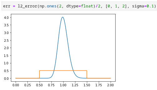
def l2_error(pmf: np.array, x_grid: np.array, sigma=0.1):
    pmf = np.array(pmf)
    x_grid = np.array(x_grid)
    assert all(pmf >= 0)
    assert np.isclose(sum(pmf), 1)
    assert all(x_grid >= 0)
    assert all(np.diff(x_grid) > 0)
    assert len(pmf) + 1 == len(x_grid)

    n_point = 2 ** 22
    tail_value = (TARGET_ERR / 100) ** 2
    min_x = lognorm.ppf(tail_value, sigma)
    max_x = lognorm.ppf(1 - tail_value, sigma)
    x_middle = np.linspace(min_x,max_x, n_point)
    x_lower_tail = np.linspace(0, min_x, n_point//1000)
    x_upper_tail = np.linspace(max_x, x_grid[-1], n_point//1000) if x_grid[-1] > max_x else np.array([])


    x_approx = np.diff(x_grid) / 2 + x_grid[:-1]
    x_approx = np.concatenate(([x_grid[0]], x_approx, [x_grid[-1]]))
    pdf_approx = pmf /np.diff(x_grid)
    pdf_approx = np.concatenate(([pdf_approx[0]], pdf_approx, [pdf_approx[-1]]))

    fy = interp1d(x_approx, pdf_approx, kind='nearest', assume_sorted=True, fill_value=(0, 0), bounds_error=False)
    x_full = np.concatenate((x_lower_tail[:-1], x_middle, x_upper_tail[1:]))
    approx_pdf = fy(x_full)

    full_pdf = lognorm.pdf(x_full, sigma)
    dx = np.diff(x_full)
    dx = np.append(dx, 0)

    plt.plot(full_pdf)
    plt.plot(approx_pdf)

    upper_tail_err_2_approx = lognorm.sf(x_full[-1], sigma)
    main_err_2 = sum((full_pdf - approx_pdf) ** 2 * dx)
    err = (upper_tail_err_2_approx + main_err_2) ** 0.5
    return err


def vanilla():
    s = 0.1
    qubits = 12
    partial = 2 ** qubits
    tail_value = (TARGET_ERR / 100) ** 2
    x_approx = np.linspace(lognorm.ppf(tail_value, s),
    lognorm.ppf(1 - tail_value, s), partial + 1)
    pmf = np.diff(lognorm.cdf(x_approx, s))
    pmf = pmf / sum(pmf)
    print(l2_error(pmf, x_approx, sigma=s))


p = [0,
     0,
     0,
     0,
     0,
     0.081,
     0.02,
     0.1,
     0.5,
     0.115,
     0.15,
     0.03,
     0.004,
     0,
     0,
     0]

x = [0.1,
     0.2,
     0.3,
     0.4,
     0.5,
     0.6,
     0.7,
     0.8,
     0.9,
     1,
     1.1,
     1.2,
     1.3,
     1.4,
     1.5,
     1.6,
     1.7]

When I try to run vanillaI get the error

Traceback (most recent call last):
File /opt/conda/lib/python3.8/site-packages/IPython/core/compilerop.py:105 in ast_parse
return compile(source, filename, symbol, self.flags | PyCF_ONLY_AST, 1)
Input In [3]
1.7]
^
IndentationError: unexpected indent

Should the 1.7 be there, or should the 1.6 have a comma after, each gives me a result. I assume it won’t change anything, but since this is new to me I am concerned I may pick up a misunderstanding somewhere,
Thanks!

Thank you for catching this. Yes, 1.6 should have a comma after it.

1 Like

I think there is a small error in the final lines of l2_error. Indeed, this line:

upper_tail_err_2_approx = lognorm.sf(x_full[-1], sigma)

computes 1-F(x), with F being the CDF of the lognormal distribution and x the upper bound of the mapping. This is thus equal to the integral from x to +inf of f(x)dx, by definition of the CDF. However, the integrand should be f^2(x) instead of f(x). Since this is the tail of the distribution, this doesn’t change the computation much though.

However, I have a problem with this method of computation, which is that, if I’m not mistaken, it tends to be slightly inaccurate for large intervals. For instance, for a single qubit in uniform superposition with mapping (0, 1, 2), the approximation function should be equal to .5 on [0, 2] and 0 elsewhere. With this method of computation, it is equal to 0 between 0 and .5, to .5 between .5 and 1.5 and to 0 elsewhere, as shown here (I’ve changed plt.plot(full_pdf) and plt.plot(approx_pdf) to plot them as function of x_full):
Screenshot_20220531_040633

For small intervals, this difference in computation is negligible. However, I do have a solution which uses a fairly large interval. I’m using this code to compute the L2 Norm:

import numpy as np
from scipy.integrate import quad

def error(p, x):
    p = np.array(p)
    x = np.array(x)
    assert all(p >= 0)
    assert np.isclose(sum(p), 1)
    assert all(x >= 0)
    assert all(np.diff(x) > 0)
    assert len(p) + 1 == len(x)
    err_squared = quad(lambda x: lognorm.pdf(x, s=0.1) ** 2, 0, float("inf"))[0]
    diff = x[1:] - x[:-1]
    err_squared += np.sum((p ** 2) / diff)
    temp = np.array([quad(lambda x: lognorm.pdf(x, s=0.1), x[i], x[i + 1])[0] for i in range(x.shape[0] - 1)])
    err_squared -= 2 * np.sum(p * temp / diff)
    
    return np.sqrt(err_squared)

This formula can be found by expanding the square within the integral and then use linearity. I do believe that this code is correct to compute the L2 norm, but I’m no expert in that field, please feel free to point me any error you’d see!

Assuming this code is correct, my problem is that a solution of mine has an error below the threshold using this code but above the threshold using the provided code. Thus my question is: can we compute the L2 norm in another way that the one which is given here, if we prove that the associated computation is correct? Or do we have to use this implementation?

Thank you in advance for your answer!

Regarding your first question, the SF function is used as an approximation for the integration to infinity since in numeric integration you need to cut somewhere.

Regarding the second question, there is indeed a mistake in the code :

x_approx = np.concatenate(([x_approx[0]], x_approx, [x_approx[-1]])
Should be:

x_approx = np.concatenate(([x_grid[0]], x_approx, [x_grid[-1]]))

Your code seems OK and you may use any method he wishes.

1 Like

Hi there!

I’ve made a simple jupyter notebook that you can open in Colab, which computes the L2 error by three different methods, one due to @QuantumSage another due to @tnemoz and the last one I wrote myself. I think mine might be the most accurate one because I used analytic equations for integrals of the lognormal distribution Though, for fine enough discretization the difference is negligible.

I mostly made this notebook to help reviewers check my solution, but post it here in case it can be useful for anyone else.

2 Likes